|
MATLAB
RESOURCES INTRODUCTION
TO QUANTUM MECHANICS
3rd
Edition
David
J Griffiths & Darrel F Schroeter
Ian
Cooper matlabvisualphysics@gmail.com CHAPTER 2 SCHRODINGER EQUATION ANHARMONIC OSCILLATOR MORSE POTENTIAL HCl MOLECULE DOWNLOAD DIRECTORY FOR MATLAB SCRIPTS simpson1d.m QMG23FA.m I will
give a simple example to illustrate the quantization of energy by solving the
Schrodinger equation with a Morse potential for the diatomic molecule HCl.
This topic is not discussed in the Griffiths text, but I will include it as
an example of the benefits of a numerical approach compared with the
analytical methods given by Griffiths. One you have solved the Schrodinger
equation using the matrix representation to find the eigenvalues and
eigenfunctions, it is a simple matter to make minor changes to the Script for
many different potential energy functions. In the
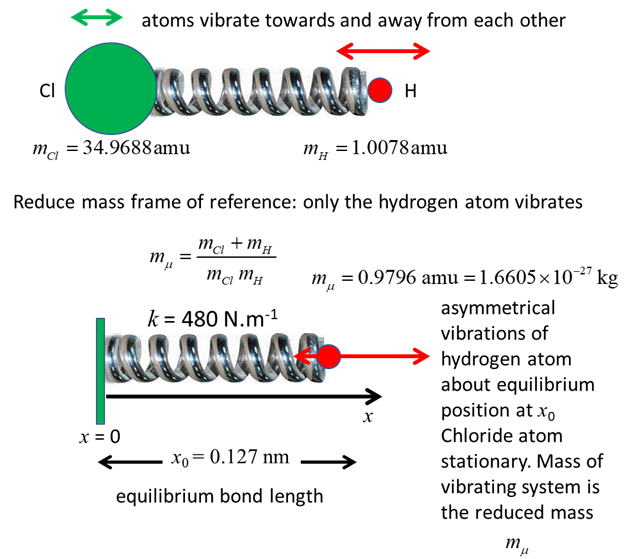
HCl molecule, the two atoms vibrate as the nuclear separation increases and
decreases as the atoms move towards and away from each other. The HCl
molecule has a permanent electric dipole moment even at the equilibrium
separation of the atoms. Therefore, vibrational emission and absorption of
electromagnetic radiation occurs due to the oscillation in the electric
dipole moment arising from the oscillations in the nuclear separation. The
selection rule for electric dipole radiation is
Fig.
1. Classical view: vibration of the
chlorine and hydrogen atoms in the HCl molecule due to their motion. Quantum
view: you don’t know anything about the trajectories of the two atoms.
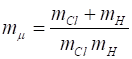
Using the reduced frame of reference, by solving the Schrodinger equation for
the system, we can only predict the probability of a given bond length. The [1D]
time independent Schrodinger equation for the single particle (lightest atom)
that is solved by the matrix method is where
the Hamiltonian operator is expressed as a matrix In solving
this Schrodinger equation, all distances are measured in nanometres and
energies in electron-volts. Full details of the Matrix Method can be viewed
at https://d-arora.github.io/Doing-Physics-With-Matlab/mpDocs/qp_se_matrix.pdf The
total energy E is due
only to the vibration of the atoms and does not relate to electronic or
rotational total energies For
small vibrations about the equilibrium bond length, we assume that the
potential energy function is parabolic and use the harmonic oscillator model.
The quantized total energy levels are
where where k is the
spring constant for the HCl molecule, k
= 480 N.m-1, The
zero-point energy is where
the fundamental frequency of vibration (classical vibration frequency) is For
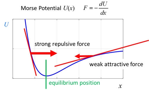
larger amplitude oscillations, the interaction between two atoms in a
diatomic molecule can be represented by a potential well function known as
the Morse potential. In the frame
of reference of the reduced mass, the bond length x
oscillates as the position of the hydrogen atom changes. Classical view: when
the hydrogen atom moves closer to the chloride atom, a large repulsive force
pushes them apart, and when they have a separation greater than the
equilibrium separation the force between the two atoms is attractive.
Fig.
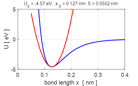
1. Morse potential. The
potential energy function
where Given
the input values for k and U0, the width
parameter is A
diatomic molecule acts essentially as a harmonic oscillator for low energy
eigenstates and is analogous to a system which executes spring-like modes of
oscillation. For higher energy states, the spacing between adjacent energy
levels decrease with increasing energy and the validity of the harmonic
oscillator is no longer valid for diatomic molecules. The
following results were generated using the Script QMG23FA.m
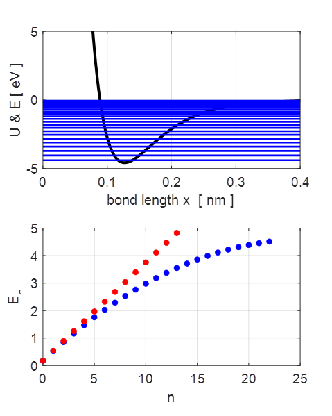
Fig.
2. The parabolic and Morse potential energy functions.
Fig. 3.
The energy eigenvalues for the parabolic
and Morse potentials. The spacing
between adjacent energy levels decreases as the energy increases for the
anharmonic potential whereas the energy levels are equally spaced for the
harmonic oscillator. Table
1. Energy eigenstates [eV]
for Morse and parabolic potentials. No. bound
states found =
23 n En [eV] Etheory [eV] 0 0.1770 0.1787 1 0.5204 0.5362 2 0.8497 0.8937 3 1.1650 1.2511 4 1.4663 1.6086 5 1.7536 1.9660 6 2.0269 2.3235 7 2.2863 2.6810 8 2.5316 3.0384 9 2.7630 3.3959 10 2.9805 3.7534 11 3.1840 4.1108 12 3.3735 4.4683 13 3.5492 4.8257 14 3.7109 5.1832 15 3.8586 5.5407 16 3.9925 5.8981 17 4.1124 6.2556 18 4.2184 6.6130 19 4.3104 6.9705 20 4.3886 7.3280 21 4.4536 7.6854 Table 2:
Transitions dn dE [eV] f [Hz] lambda [nm] (0,
1) 0.3434 8.303e+13 3611 (1, 2) 0.3294 7.964e+13 3765 (2, 3) 0.3153 7.624e+13 3932 (3, 4) 0.3013 7.285e+13 4115 (4, 5) 0.2873 6.947e+13 4316 (5, 6) 0.2733 6.609e+13 4536 (6, 7) 0.2593 6.271e+13 4781 (7, 8) 0.2454 5.933e+13 5053 (8, 9) 0.2314 5.595e+13 5358 (9, 10) 0.2174 5.258e+13 5702 (10, 11) 0.2035 4.921e+13 6092 (11, 12) 0.1896 4.584e+13 6540 (12, 13) 0.1756 4.247e+13 7059 (13, 14) 0.1617 3.910e+13 7668 (14, 15) 0.1478 3.573e+13 8390 (15, 16) 0.1338 3.236e+13 9263 (16, 17) 0.1199 2.900e+13 10339 (17, 18) 0.1060 2.563e+13 11698 (18, 19) 0.0921 2.226e+13 13469 (19, 20) 0.0781 1.889e+13 15866 (20, 21) 0.0650 1.572e+13 19073 (21, 22) 0.0585 1.414e+13 21203
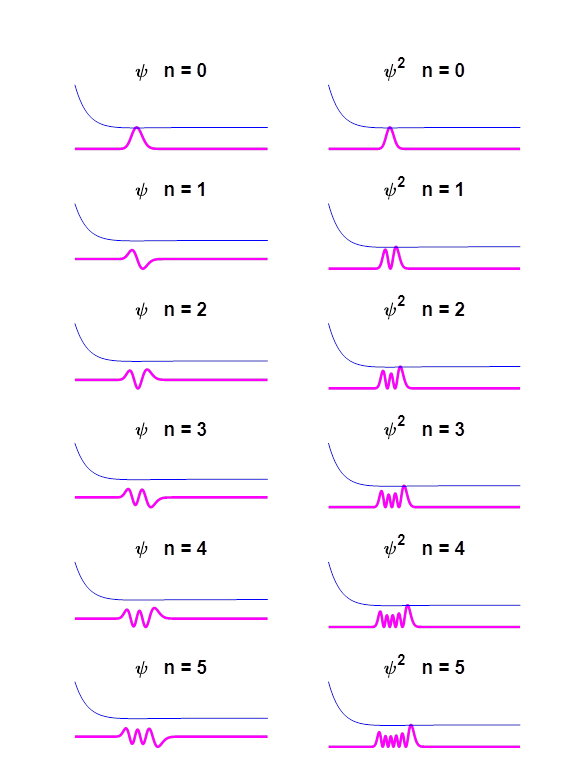
Fig.
6. Eigenfunctions for the Morse
potential for eigenstates n = 0 to n =5. Eigenstate
n
= 4
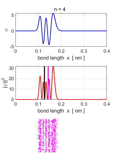
Fig.
7. Eigenstate n = 4.
Eigenfunction and probability density plots. Centre plot: black vertical line
shows the equilibrium separation and the magenta vertical line the
expectation value for the separation. Note: the expectation value for the
separation is greater than the equilibrium position. Single
stationary state computations Stationary
State n = 4 Total
energy EM = -3.1037
eV Total
Probability = 1 <x>
= 0.1433 nm <x^2>
= 0.0211 nm^2 <ip> = -9.7575e-40 N.s <ip^2>
= 3.4459e-46 N^2.s^2 deltax,dx =
2.4587e-11 m deltap,dp =
1.8563e-23 N.s (dx dp)/hbar
= 4.33 Uncertainty
Principle (dx dp)/hbar
>= 0.5
satisfied <U>
= -3.7665 eV <K>
= 0.6608 eV <E>
= -3.1058 eV <K>
+ <U> = -3.1058 eV Probability
x < x0 = 0.3155 Probability
x > x0 = 0.6845 Eigenstate
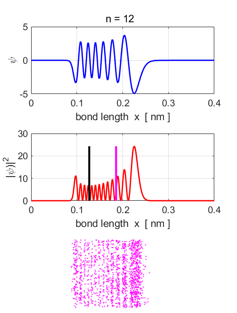
n = 12
Fig.87. Eigenstate n = 12.
Eigenfunction and probability density plots. Centre plot: black vertical line
shows the equilibrium separation and the magenta vertical line the
expectation value for the separation. Note: the expectation value for the
separation is greater than the equilibrium position. Single
stationary state computations Stationary
State n = 12 Total
energy EM = -1.1965
eV Total
Probability = 1 <x>
= 0.1855 nm <x^2>
= 0.0366 nm^2 <ip> = 4.1326e-40 N.s <ip^2>
= 5.9251e-46 N^2.s^2 deltax,dx =
4.6504e-11 m deltap,dp =
2.4342e-23 N.s (dx dp)/hbar
= 10.73 Uncertainty
Principle (dx dp)/hbar
>= 0.5
satisfied <U>
= -2.3402 eV <K>
= 1.1362 eV <E>
= -1.2041 eV <K>
+ <U> = -1.2041 eV Probability
x < x0 = 0.1752 Probability
x > x0 = 0.8248 |