|
Ian Cooper matlabvisualphysics@gmail.com A COMPUTATIONAL APPROACH TO ELECTROMAGNETIC THEORY ELECTRIC DIPOLE RADIATION Generation of EM waves DOWNLOAD
DIRECTORIES FOR MATLAB SCRIPTS cemEDR01.m E field and B field
plots generated by an oscillating electric dipole. Vector diagrams and
contour plots. cemEDR02.m E field, B field,
Poynting vector plots generated by an oscillating electric dipole. Animation of E field and B field as a
function of the radial displacement from the dipole. cemEDR03.m Animation of the E field
in the YZ plane. cemEDR04.m E-field and B field as
functions of radial displacement and polar angle. DrawArrow.m This function is used to
add arrows to a plot. zT = 2+2.5i; zTmag
= 1.3; zTA = pi/2+atan2(2.5,2); HL = 0.2; HW = 0.2; LW = 2; col =
[0 0 1];
DrawArrow(zT, zTmag, zTA, HL, HW, LW, col) % B zT Tail of the arrow expressed as a
complex number; zTmag magnitude of the vector; zTA angle of the vector w.r.t.
“X axis” in radians;
HL arrow head
length; HW arrow head width; LW line width; col colour of arrow. INTRODUCTION Maxwell's equations
imply that classical electromagnetic radiation is generated by accelerating
electrical charges. As an example, we will consider the generation of
electromagnetic waves from an oscillating
electric dipole. Although this is an idealized system, it provides
a basic building block for constructing realistic sources of radiation from
antenna systems. An infinitesimal electric dipole oscillating at a single
frequency is known as an Hertzian dipole. Matlab can be used extensively
to de-mystify much of the complicated mathematics describing the generation
of electromagnetic waves. Such an approach may be helpful for students to
understand better radiation phenomena. ELECTRIC DIPOLE Consider two point-like
particles located on the Z axis, and close to each other on opposite sides of
the Origin. Suppose an electric current (charge) flows between the two
particles. The charge oscillates on each particle oscillates as (1A)
(1B)
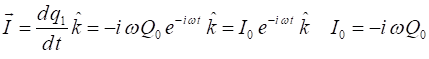
The current between the
charges is (2)
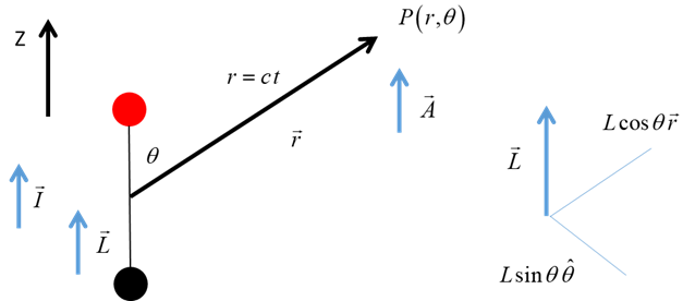
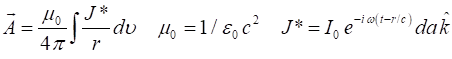
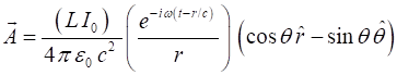
We can calculate the
vector potential
Fig. 1. Radiating dipole: dipole moment Wave parameters: Vector potential:
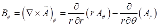
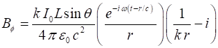
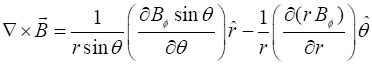
(3) The B-field is easy to
calculate since
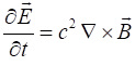
(4A) (4B) The electric field can
be obtained from one of Maxwell’s equations in free space
Using the fact that
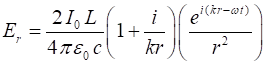
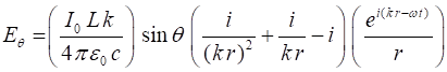
The electric field is
(5A)
(5B)
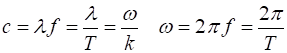
To convert spherical
coordinates to Cartesian coordinates use
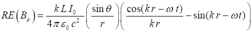
(5C) (5D) (5E) The field equation all
involve the phase factor
In the far field region
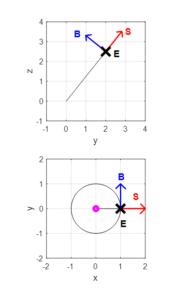
Fig. 2. The E and B fields components are
perpendicular to each other and to the direction of energy transfer (Poynting
vector – radial direction The energy radiated from
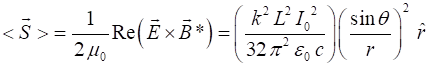
the dipole is given by the Poynting vector (6A)
and the instantaneous
Poynting vector as (6B)
There is zero radiation
along the axis of the dipole MODELLING The usual textbook
treatment is mainly mathematical with images or detailed plots of the fields
barely shown. Using Matlab as a
tool, you gain a much greater insight to EM wave generation than with the
mathematics alone. Also, much of
the algebra can be avoided. For example, given the electric field as a
complex quantity, there is no need to do all the “hard work” in
finding the real part. The electric field given by equation (5D) can be
computed and only the real part plotted. The many figures below indicate some
of the possibilities of giving a more visual picture of the EM radiation
emitted from an electric dipole. The default wavelength for the modelling is
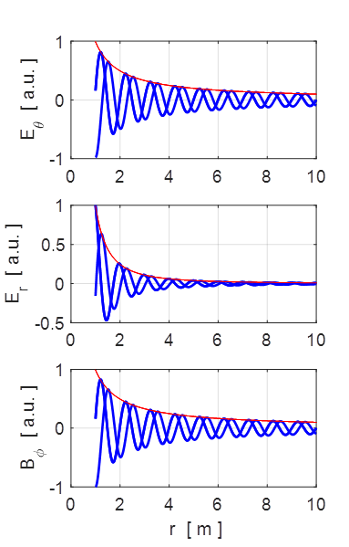
Fig. 3A. Plots of the components of the E and B
fields at time
Fig. 3B. Plots of the components of the E
and B fields at times
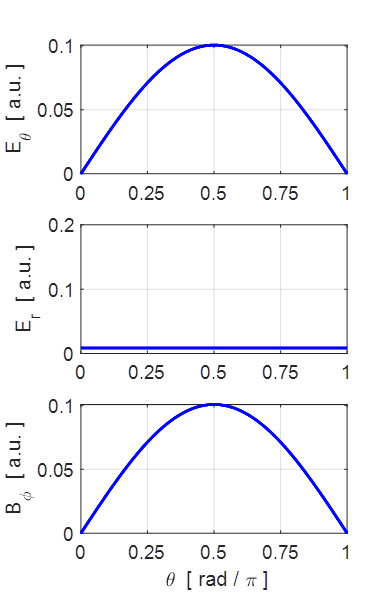
Fig. 4. The E and B field strengths
depend upon the polar angle
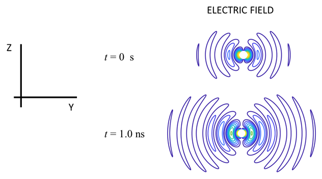
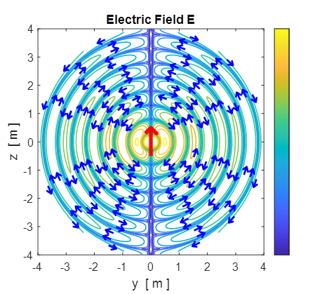
Fig. 5A. The electric field lines
displayed in the YZ plane at time t = 0 and t = 1.0 ns (period T = 3.3356 ns). cemEDR01.m
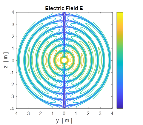
Fig. 5B. The electric field lines
displayed in the YZ plane as a contour plot of During one period, the
loop of E shown closest to the source moves out and expands to become the
loop shown farthest from the source.
cemEDR01.m
Fig. 5C. The electric field lines
displayed in the YZ plane. The electric field values are scaled to better
observe the pattern of the E field lines. Blue
arrows of unit length some the direction of the E field as random
points. (could not get
Matlab’s quiver or streamline functions to give the vector field) cemEDR01.m
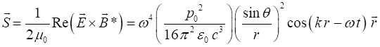
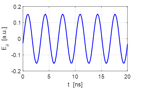
Fig. 6. The time variation of the E
field at a point
Fig. 7. Animated view of the E and B fields in
the equatorial plane. The fields propagate at the speed of light in a radial
direction away from the dipole. The red curves for
the envelopes show the fields fall off as
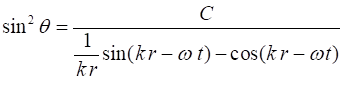
Fig. 8. Animated view of the E field
lines in the YZ plane. The E field lines were calculated from the equation
Different values of C
correspond to different field lines.
Propagation of the electric field lines, whose time dependence is
periodic with a period of
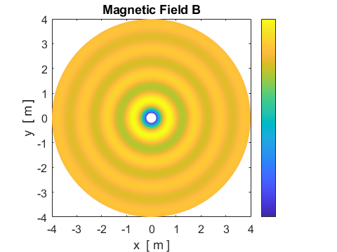
Fig. 9. B field in the XY equatorial
plane cemEDR01.m
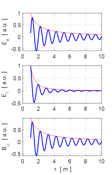
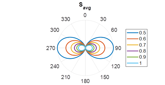
Fig. 10. The Poynting vector. Each
coloured line corresponds to different radial distances from the dipole (0.5
m to 1.0 m). The image gives the distribution of radiated power from an
Hertzian dipole. The current in the dipole is oriented along the z axis. The
distance of a point on the curves from the Origin indicate the relative power
density in the direction from the Origin to a pont on the curve. There is
zero radiation along the axis of the dipole There is zero cemEDR02.m SUMMARY In the near field of the
oscillating dipole, the energy flow alternates regularly between outward and
inward directions since the E and B field are 90o out of phase due
to oscillating charges and current.
The result is that the net energy flow is zero and this pulsating
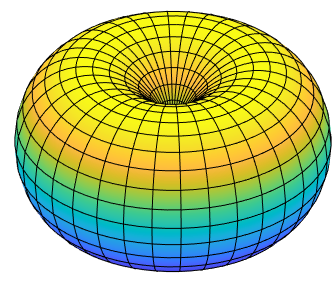
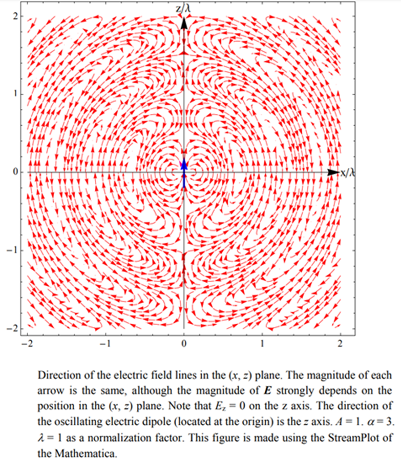
field falls off as The following plot is
from https://bingweb.binghamton.edu/~suzuki/SeniorLab_pdf/16_Radiation_from_electric_dipole.pdf I cannot produce such a
nice figure in Matlab.
|