|
NUMERICAL ANALYSIS
OF OPTCIAL AND ELECTROMAGNETIC PHENOMENA PROPAGATION OF ELECTROMAGNETIC WAVES IN FREE SPACE Ian Cooper matlabvisualphysics@gmail.com DOWNLOAD
DIRECTORY FOR MATLAB SCRIPTS op_001.m Plots and an
animation of a plane wave propagating in the +Z direction. The wavelength of
the EM wave is changed in the INPUT section of the script and should be in
the range for visible light (380 nm to 780 nm). The plots are color coded to match the color
of the light by calling the script colorCode.m. op_002.m
[2D] animation of
a plane wave propagating in +Z direction. opLE1001.mlx LIVE EDITOR:
Vector calculus applied to plane EM waves using the Symbolic Toolbox. THE WAVE EQUATION
IN FREE SPACE Electromagnetism is the fundamental theory that
underlies most of optics associated with wave phenomena. Maxwell’s equations
provide the basic information needed to describe electromagnetic phenomena.
Equation 1 gives a summary of Maxwell’s equation for free space
(vacuum). (1A) Gauss’s
Law
(1B)
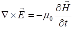
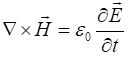
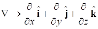
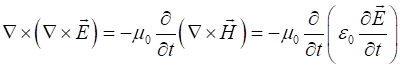
(1C) Faraday’s law
(1D) Ampere’s Law
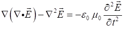
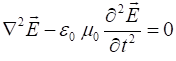
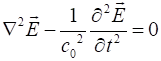
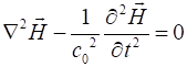
We can use Maxwell’s equation to derive the wave equation
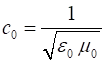
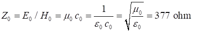
using the identify for the vector (2) The speed of light in
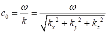
free space is (3) The speed of light in
free space is defined to be So, the wave equations
for the electric and magnetic fields are (4A) (4B) |
|
LIVE EDITOR opLE1001.mlx Vector
Calculus We can use the Live Editor in Matlab to symbolically evaluate various calculus
operators. Consider the vector field syms x
y z % Vector field A =
[x^2*y*z, y^2*z*x, z^2*x*y] % Cartesain system vars = [x y z] % Curl R1 =
curl(A,vars) R2 =
curl(R1,vars) % Divergence R3 =
divergence(A,vars) % Gradient R4 =
gradient(R3) % Laplacian R = R4
- R2 R1 = R2 = R3 = R4 = R = Using the symbolic
functions in the Live Editor, you no longer need to do all the tedious
algebra manipulations for many calculus operations. |


|
PLANE HARMONIC (MONOCHROMATIC)
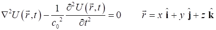
WAVES The vectors for the electric field (5) where It is often convenient to assume that the wavefunction
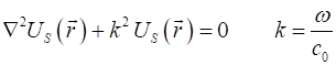
(6) By substitution of equation 6 into equation 5, we can derive the Helmholtz
equation
(7) The Maxwell equations 1C and 1D, for harmonically varying fields,
reduce to
(8C)
(8D) We will consider the special case of a plane harmonic electromagnetic wave propagating in the +Z direction, where
(9)
By direct substitution of equation 9 into equation 5, it is to verify
that the electric field given by equation 9 is a solution to the wave equation (5) provided that the ratio of
the constants
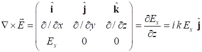
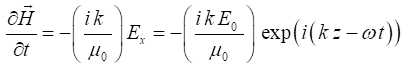
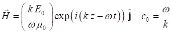
(10) We can then substitute equation 9 into the Maxwell equation 1C to
find the magnetic field component of our plane harmonic electromagnetic wave
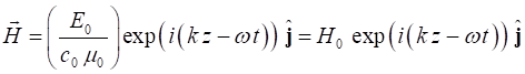
(11)
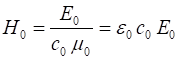
The ratio
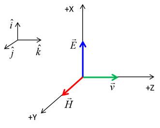
Our plane harmonic electromagnetic wave is a transverse wave
propagating in the +Z direction with the electric field varying in the +X
direction and the magnetic field varying in the +Y direction. The vibrations
of the electric field and the magnetic field are in phase at the same
frequency at all times. This type of wave, in which the electric field vector
is always parallel or antiparallel to a fixed direction is called a plane-polarized
wave. For the solution given by equation 9, the plane of
polarization is the XY plane (figure 1).
Fig. 1. A plane electromagnetic wave
propagating in the +Z direction. The direction of propagation and the
directions of the oscillations for the electric field and magnetic field are
mutually orthogonal. The plane of polarization is the XY plane.
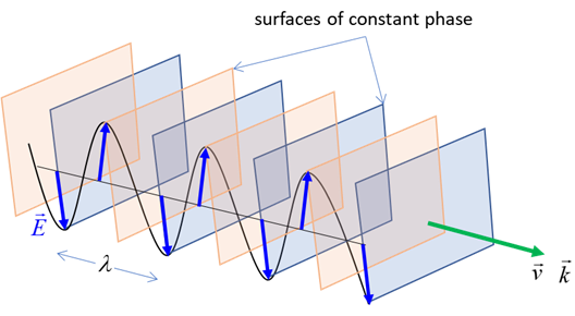
Fig. 2. Wavefronts of a plane wave travelling
in [3D] space. The direction of propagation is perpendicular to the planes of
constant phase. The wave advances such that the phase in the plane perpendicular to
the direction of propagation remains constant.
We can differentiate this expression for the phase with respect to
time t
But
(10) When the phase of the wave increases by For one cycle, where the wave advances a distance
(12)
For one cycle, where the time advances by T and the electric field values at times
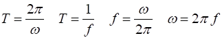
(13) T is the period and is the time for one
complete oscillation. The reciprocal of the period T is the frequency f and is the number of cycles per unit
time. T period
[s] f frequency
[Hz] Hence, the wave travels a distance
(10) For a plane wave given by the phase velocity is The solutions of electromagnetic field problems with an arbitrary time
dependence can be constructed by using Fourier
transformation theory. |


|
LIVE EDITOR: Vector Calculus opLE1001.mlx We can use the Live Editor to verify equation 9 is a solution of the
scalar wave equation 6. syms k z w t clc E = exp(-1i*(k*z
- w*t)) v = w/k % LHS = d2E_dtz2 RHS = (1/v^2)*d2E/dt2 LHS = diff(E,z,2) RHS = (1/v^2)*diff(E,t,2) E = v = LHS = RHS = |
|
Returning now to the [3D] wave equation (5), it is readily verified
that equation (5) is satisfied by the three-dimensional plane harmonic
wavefunction
(14) where the position vector is
and the propagation vector is given by its components
Constant values of the phase
and the propagation vector
(10)
The wavefunctions are expressed as complex function. However, it is
only the real
part of these functions that represent actual physical quantities. |
|
ENERGY FLOW AND THE POYNTING VECTOR The rate at which energy is transferred by a plane wave is given by
the Poynting
vector S [W.m-2]
which is defined as the cross produce of the electric and magnetic fields
(15)
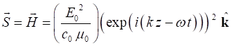
For our harmonic wave
(9)
(11)
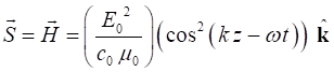
Taking the real part for the actual value of the Poynting vector
The average value of the cosine squared is equal to ½. Hence,
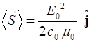
the time average value of the Poynting vector is
The flow of energy is in the same direction in which the wave
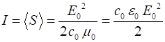
propagates. The magnitude of the average Poynting vector is called the intensity
(16) Thus, the rate of energy flow is proportional to the square of the
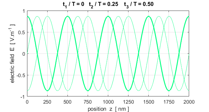
amplitude of the electric field. The temporal and spatial variations of the electromagnetic field for
a 1.0 mW plane monochromatic wave propagating in
the +Z direction with its plane of polarization directed long the X-axis are
displayed in figure 3, 4 and 5 for green light
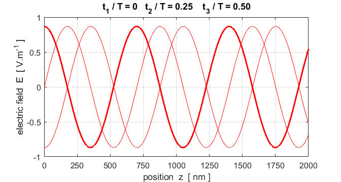
Fig. 3. A plot of the electric field as
a function of position at three time steps. Note: the wave advances to the
right a distance of one wavelength in a time interval of one period. op_001.m
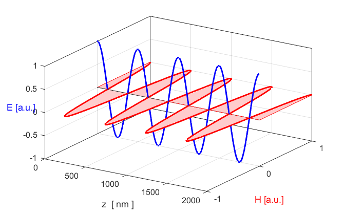
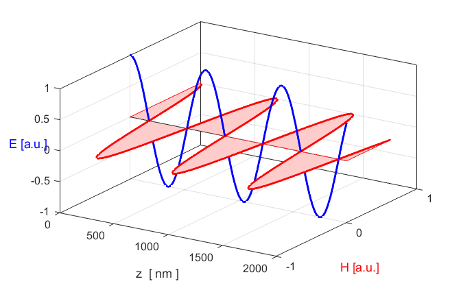
Fig. 4. The oscillations of the electric field
and magnetic field are in phase and perpendicular to each other and
perpendicular to the direction of propagation as shown in figure 1. op_001.m
Fig. 5. Animation of the vibration of
the electric field as the wave propagates in the +Z direction. From the plot,
you can verify the relationship Figure 6 shows the electromagnetic fields for red light
Fig. 6. The electromagnetic fields for a plane
wave with It is easy to create an animation of a plane wave propagating in
two-dimensions. The [2D] version of a plane wave shows how the wavefronts are
straight lines (lines of constant phase) that move in the direction of
propagation. In [3D], you can think of the straight lines of constant phase
as planes extending out of the screen and moving in the direction of
propagation.
Fig.
7. [2D] view of a plane
wave. op_002.m |

|
Live Editor Poynting
vector
opLE1001.mlx Calculation
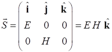
of the Poynting vector for a plane wave polarized in the X-direction. syms k
z w t E0 mu0 c0 E
= [E0*exp(1i*(k*z - w*t)), 0, 0] H
= [0, E0/(c0*mu0)*exp(1i*(k*z - w*t)), 0] S
= cross(E,H) E = H = S = |
|
|