|
MICHELSON INTERFEROMETER Fringe Patterns Ian Cooper Email: matlabvisualphysics@gmail.com |
|
MATLAB SCRIPTS opMichA.m Plane wave illumination of Michelson Interferometer. The mirrors are aligned perpendicular to the beam. An animation is displayed of the view on a detector screen as the distance between the mirrors is changes. The Michelson Interferometer can be used to measure small distance and an example of measuring plant growth is used. Calls the function ColorCode.m. opMichB.m Plane wave illumination of Michelson Interferometer with one of the mirrors tilted by a small angle w.r.t. the X axis. A vertical fringe pattern is shown on the detector screen. Calls the function ColorCode.m. opMichC.m Point source illumination of Michelson Interferometer produces circular fringes. Input parameters: wavelength and virtual source separation. Calls the function ColorCode.m. |
|
MICHELSON
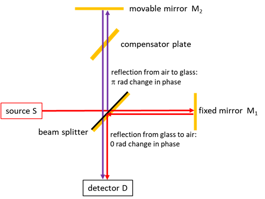
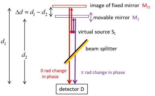
INTERFEROMETER In the Michelson interferometer, light from a source is split into two beams at a beam splitter (partially reflecting mirror). One beam travels to a fixed mirror M1 and is reflected back to the beam splitter while the other beam is reflected from a movable mirror M2 back to the beam splitter. The two beams recombine and are then detected as shown in figure 1. The two beams must be mutually coherent for interference fringes to be observed. This process is known as interference by division of amplitude. It is assumed that the beam splitter divides the two beams equally and is oriented at 45o to the source beam.
Fig. 1. Michelson interferometer. When the two
beams combine at the detector, there is a A linear optical
equivalent of the Michelson interferometer helps to understand the
optical path differences (figure 2). The mirror M1 is replaced
with its virtual image M1I
seen when looking into the beam splitter from the source. The source aperture
is replaced by its virtual image SI
as seen looking into the beam splitter from the position of mirror M2.
The detected interference pattern is the same as would be generated by a
source SI
that is reflected from two distinct mirrors M2 and M1I, separated by a distance
Fig. 2. Linear optical equivalent arrangement of the Michelson interferometer. For the rays that travels along the central path of the interferometer,
the optical path difference between the light reflected from the two mirrors
M1I and
M2 is At the centre of the detector
destructive interference – dark spot
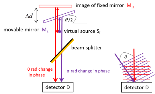
constructive interference – bright spot Illumination by a monochromatic plane wave Assume the two mirrors
M1I and M2 are
illuminated by an incident plane wave. The mirror M2 is titled at an angle
Fig. 3.
Illumination by monochromatic waves with mirror M2 titled at an angle
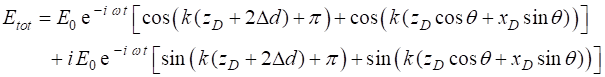
The electric fields
for the two plane waves at the point
(1A)
(1B)
Then, the resultant
electric field
(3)
The
intensity
and after much algebra
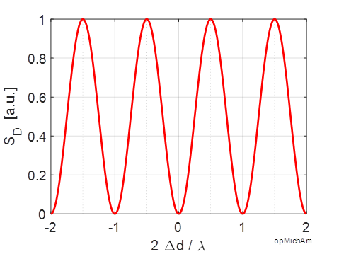
(4) Mirrors precisely aligned at right angles to the beam If the two
mirrors are precisely parallel
and the whole area of the screen will be uniformly illuminated. The screen will be dark when the difference in the optical path lengths of the two beams are an integral multiple of a wavelength and bright when the there is an odd multiple of a half-wavelength (figures 4 and 5).
Dark (destructive interference)
Bright (constructive interference)
Fig. 4. The detector screen SD
intensity as a function of the optical path length difference
Fig. 5. Variation in the detector screen intensity as the position of mirror M2 changes. Figure 5 shows that the number |
|
Example Plant Growth The Michelson interferometer can
be used to measure small displacement accurately. For example, it is possible
to measure the growth rate of a plant. The plant was attached to the movable
mirror M2 and its position was adjusted to give a black field of
view on the detector screen. A helium-neon laser was used with a wavelength
0f 632.8 nm. As the plant grew, the distance between the mirrors increased.
So, the fringe pattern changed in a manner as observed in the animation of
figure 5. In an 8.0 hour period, The calculation can be done using the Script opMichA.m %
Plant Growth Calculation %
wavelength [m] wL =
632.8e-9; % Time
interval [h] dt = 8; %
Number of fringes nf = 3420; %
distance moved by plant on mirror 2 [mm] dP = (nf * wL /2) * 1e3; %
rate of growth [mm/h] dPdt = dP/dt; disp('Inputs ') fprintf(' wavelength = %3.1e m
\n',wL); fprintf(' time interval = %3.1f h
\n',dt); fprintf(' fringes = %3.0f \n',nf); disp('Outputs ') fprintf(' growth distance = %3.5f mm \n',dP); fprintf(' rate of growth = %3.5f mm/h \n',dPdt); Inputs wavelength = 6.3e-07 m
time interval = 8.0 h
fringes = 3410 Outputs growth distance = 1.07892 mm rate of growth = 0.13487 mm/h Inputs fringes = 3415 Outputs growth distance = 1.08051 mm rate of growth = 0.13506 mm/h Inputs fringes = 3420 Outputs growth distance = 1.08209 mm rate of growth = 0.13526 mm/h Growth
rate = |
|
Mirror M2 rotated
about the Y axis Waves reflected by
M2 at an angle The intensity of the detector
screen is due to the interference of the two plane waves. The wavefronts from
the reflection from mirror M1I are parallel
to the screen, while the wavefronts from the reflection from mirror M2
are tilted at an angle to the screen (figure 3). The resultant interference pattern
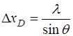
shows a series of vertical bright and dark equally spaced fringes. The angle The fringes are given by the equation (4) Using equation 4, the spacing
(5) When
the fringes disappear and the screen becomes uniformly illuminated as described above. The fringe separation becomes smaller as the wavelength decreases and the tilt angle becomes larger. When mirror M2 is moved, then the fringes move in a horizontal direction across the detector screen. The Michelson interferometer is modelled for plane wave illumination with the Script opMichB.m and the Live Editor Script opMichBLE.mlx. Using the Live Editor with the numeric sliders, one can change the wavelength, mirror separation distance and the tilt angle and immediately observe the changes in the interference pattern.
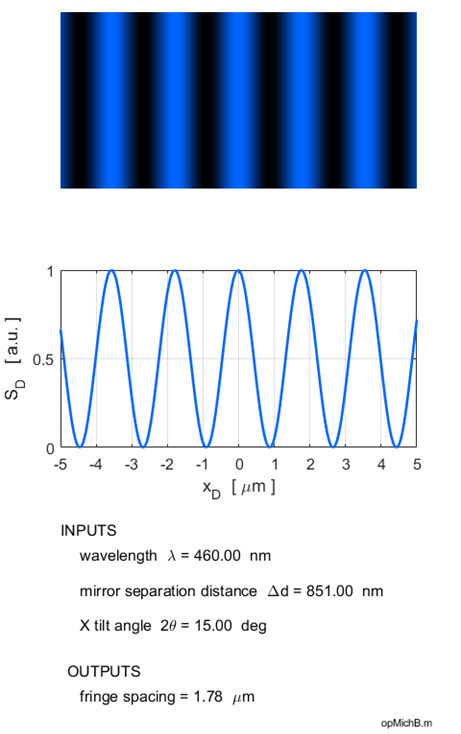
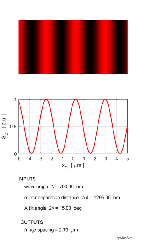
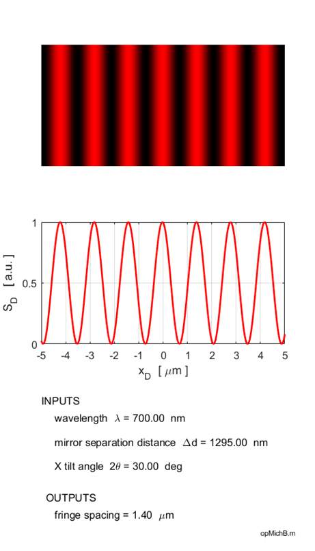
Fig. 6. Fringes of equal thickness are
generated when mirror M2 is tilted. The fringe spacing is reduced as the
wavelength is decreased and the tilt angle is increased as predicted by
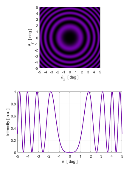
equation 5. Illumination by a monochromatic point source You can calculate the fringe pattern for point source illumination using the script opMichC.m. The input parameters are the wavelength, the distance between the virtual sources and the maximum viewing angle. The spherical waves produce circular fringes on a viewing screen. A dark spot is located at the centre of the fringe pattern if the distance between the virtual source points
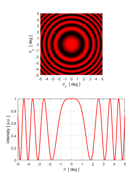
A bright spot is located at the centre of the fringe pattern if the distance between the virtual source points
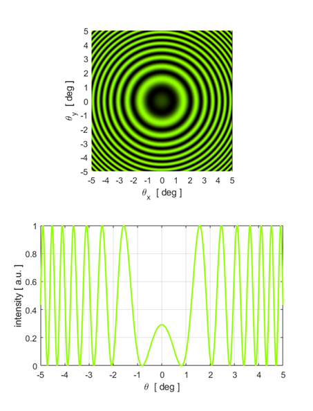
m is called the order of the fringe. Three examples are shown below.
Fig.
7A. Circular fringe pattern:
Fig.
7B. Circular fringe pattern:
Fig. 7C. Circular fringe pattern:
|