|
COMPUTATIONAL NEUROSCIENCE GEOMETRICAL
METHODS OF ANALYSIS OF [1D] DYNAMICAL SYSTEMS Ian Cooper Any
comments, suggestions or corrections, please email me at matlabvisualphysics@gmail.com |
|
MATLAB np002B.m The function ode45 is
used to solve the equation of motion to calculate the time evolution of the
membrane potential for different models.
To obtain the plots in this article, the Script needs to be modified
by commenting and uncommenting the close all and hold on statements and by changing the plot parameters.
The Script models the nonlinear dynamical system for a leak current / fast
sodium ion current to simulate the upstroke of an action potential. For the
leak current model, let GNa = 0 (zero sodium
conductance). np001.m Simplified version of Script np002B.m for leak current only. Comparison of numerical and
analytical solutions. np001A.m Simplified versions of Script np002B.m for leak current / sodium ion current with a constant
sodium conductance. np003.m Script can
be used to give the phase portrait plot and time evolution of the state
variable x
for systems of the form Cell1: Phase Portrait Plot: Define function in Cell 1 Cell 2: Time Evolution of State Variable:
Solve equation of motion Cell 3: Define function in Cell 3 at end of
Script Different functions can be modelled by
changing the Script in Cells 1 and 3. Includes code for finding the zero of a
function. np003A.m An extension of Script np003.m for systems of the form |
|
GEOMETRICAL METHODS OF ANALYSIS OF [1D] DYNAMICAL SYSTEMS In this section will start our
study of the geometrical methods of analysis of [1D] dynamical systems, that
is, systems having only one variable. This section is linked to Chapter 3 of Izhikevich’s book. However, the results given in
this chapter using Izhikevich’s input data could
not be reproduced using my Scripts. I had to change the numerical values used
for the simulations. In general, [1D] dynamical systems
are described by ordinary differential equations of the form
where V is a scalar time-dependent
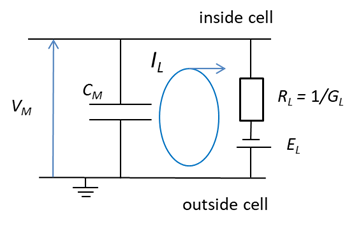
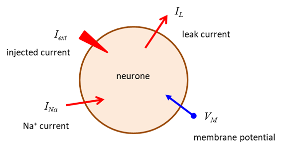
variable which represents the state of the system. V is called a state variable. Since Space-clamped membrane having only a ohmic leak current A space-claimed membrane is one in
which the membrane potential is fixed by an experimenter and an external current
exerted into the neurone. The space-clamped condition is Possibly, the simplest [1D]
dynamical system we can look at is a neurone which has only an ohmic leak
current.
The equation of motion to be
solved is (9A) (9B) (9C) The membrane potential VM is the single time-dependent variable. The
membrane capacitance CM, the leak conductance GL, and the leak reversal potential EL are all constants. The explicit analytical solution
of equation 9C is (9D) where the initial value of the membrane
potential is If the membrane potential is disturbed
from its rest potential (EL) then it will decay back to its resting
level and the membrane current will tends towards zero. Equation 9C is solved numerically
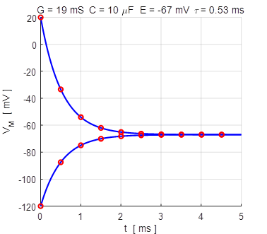
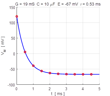
(ode45 function) and analytically using the Script np001.m with the input parameters: % conductance [19e-3 S] G = 19e-3; % Membrane capacitance [10e-6
F] C = 10e-6; % Reversal potential / Nernst
potential [EL = -67e-3 V) E = -67e-3; % Simulation time [5] N = 10; % Initial membrane
voltage [0 V] V0 = 20e-3; The Script can be run for different initial values of the membrane potential Vo and one can compare the numerical and analytical solutions as shown in figures 4A and 4B.
Fig. 4A. The membrane potential as a
function of time for two different initial values of the membrane potential.
The red dots show the analytical
solution and the blue curve, the numerical solution. np001.m
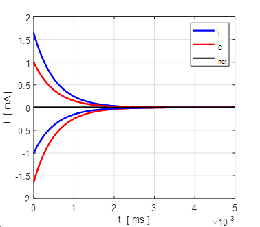
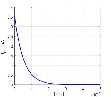
Fig.
4B. The membrane currents
as function of time for two different initial values of the membrane
potential. A
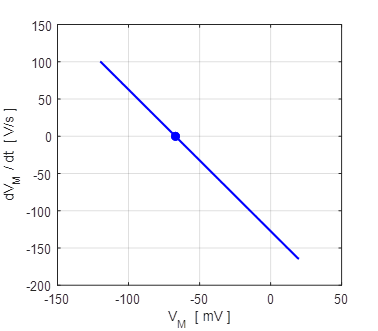
phase portrait is a geometric representation of the trajectories of a
dynamical system in the phase plane. Each set of initial conditions is
represented by a different curve, or point. Phase portraits are an invaluable
tool in studying dynamical systems. The phase portrait for our neuron model
is a plot of the time derivative of the potential against the potential is a
straight line (figure 5). For all initial conditions, the membrane potential
will be pulled to the reversal potential
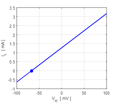
Fig. 5A. The straight line corresponds to the phase portrait plot for an ohmic element. The blue dot shows the reversal potential when time derivative of the potential becomes zero. np001.m Also, a useful plot is the I-V characteristic curve as shown in figure 5B.
Fig. 5B. I-V characteristic curve for two different initial conditions (-100 mV and +100 mV). The blue dot represents the equilibrium point (stable equilibrium) where the final current is zero and the membrane potential equals the leak reversal potential. A positive value of the current indicates an outward current to decrease the membrane potential while a negative current is an inward current which increases the membrane potential. The straight means that the conductance is constant and the slope of the line gives the numerical value of the conductance (G = 19 mS). In our simple model, the steady-state solution of the equation of motion 9C is (10) The
point
Fig.6. The initial membrane voltage is reduced to the leak reversal potential (steady-state) by a net outward current (net movement of positive charge from inside to outside the cell membrane) that hyperpolarizes the membrane. If the initial value of the membrane potential was less than the reversal potential, then a net inward current would depolarize the membrane. In
the qualitative analysis of any dynamical system it is important to find the
equilibria or rest points, i.e., the values of the state variable where F(V) = 0 and V
is an equilibrium value. At each such point We can add to our model a sodium ion channel which has a constant conductance. The equation of motion for our model is (11) Equation (11) is solved using the Script np001A.m with input parameters % conductance
[19e-3 74e-3 S] GL = 19e-3; GNa = 74e-3; % Membrane
capacitance [10e-6] C = 10e-6; % Reverse potential
/ Nernst potential [EL = -67e-3
V ENa
= 60e-3) EL = -67e-3; ENa =
60e-3; % Simulation
time [13-3 s] tMax = 1e-3; The results are displayed in figures 7, 8 and 9.
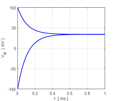
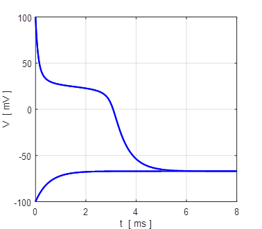
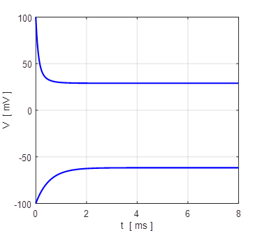
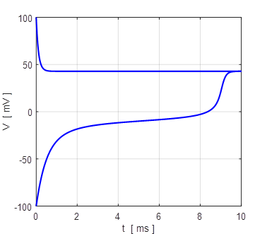
Fig. 7. The membrane potential VM
evolves to its equilibrium value of +34 mV from an initial value of +100 mV
and -100 mV.
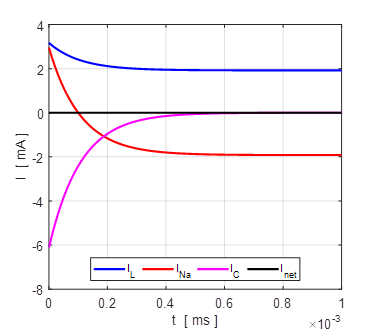
Fig. 8. The time evolution of the membrane currents. At equilibrium, the outward leakage current is balanced by the inward Na+ current. Initial membrane potential is +100 mV. np001A.m
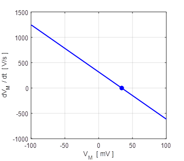
Fig. 9A. Phase portrait plot. The stable equilibrium point is (34, 0). np001A.m The I-V characteristic plot is shown in figure 9B for the leak and sodium ion currents.
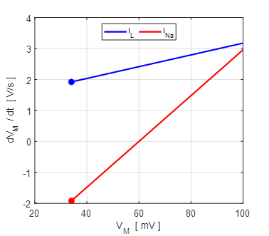
Fig. 9B. I-V characteristic plot for the leak current (blue) and sodium current (red). When a steady-state is reached (shown by the two dots), the outward flow of the leak current is balanced by the inflow of sodium ions. Space-clamped membrane having only a ohmic leak current and sodium ion
channel: Leak / fast Na+ model
We can extend our simple model further my including
a voltage dependent sodium ion channel and not an ohmic Na+
channel. The conductance of an ion channel is time and voltage sensitive. We
will consider a space-clamped membrane having a leak current and a fast
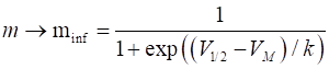
voltage-gated sodium ion current having only one variable m. The gating process is assumed to be instantaneous
such that the variable m is equal to
its asymptotic value minf where (11)
Fig. 10.
The activation function The dynamics
of the system is described by the equation (12) The Script np002B.m can be used to solve equation 12 using the ode45
function. Model parameters can be changed in the input section of the Script.
Typical values are: % INPUTS
>>>>>>>>>>>>>>>>>>>>>>>>>>>>>>>>>>>>>>>>>>>>>>>>>>>>>>>>>>>>>> % conductance [19e-3 74e-3 S] gL = 19e-3; gNa = 74e-3; % Membrane capacitance
[10e-6] C = 10e-6; % Reverse potential / Nerest potential
[EL = -67e-3 V ENa = 60e-3] EL = -67e-3; ENa
= 60e-3; % Simulation time [5e-3 s] tMax =
10e-3; % Initial membrane
voltage [0 V] unstable equilibrium 6.672903e-3 V0 = 6.5672903e-3; % V1/2 [V] k [V] Vh = 19e-3;
k = 9e-3; % External current input [A] Iext =
0.60e-3; For certain input parameters, there is a
“negative conductance” and our model can show a few interesting nonlinear
phenomena, such as bistability (co-existence of the
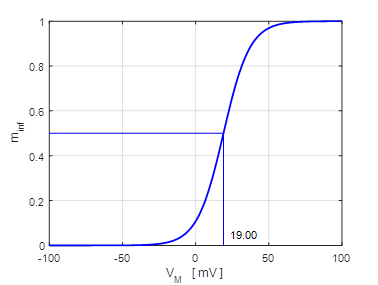
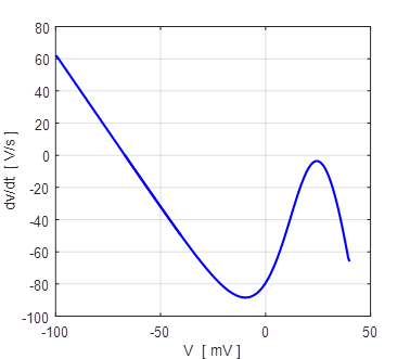
resting state and excited state). The phase portrait
plot for the solution to equation 12 for different initial conditions is
shown in figure 11 which shows three distinct equilibrium points where
Fig.
11. There are two
attraction domains which are separated by the unstable equilibrium point at
+6.6729 mV. For any initial membrane potential, the membrane potential
will converge to one of the two stable
equilibrium points: ‑ 34.5 mV (rest state) or + 38.8 mV
(excited state). The red arrows show the attraction
domains. An attraction domain of an attractor is the set of all initial
conditions that lead to the attractor.
np002B.m
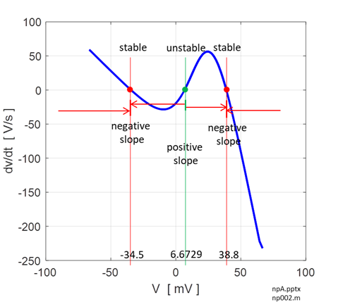
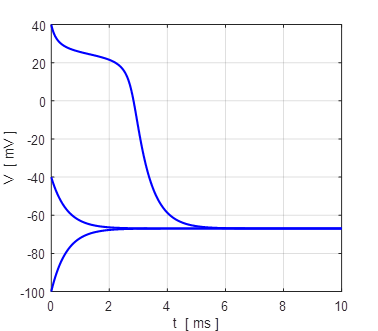
Fig. 12. Voltage trajectories for the leak / fast sodium ion model for different initial conditions. For all initial values of the membrane potential greater than the unstable membrane potential, the membrane potential is attracted to the excited state and for initial values less than the unstable equilibrium potential, the membrane potential is drawn to the resting state (bistability). The attraction to a stable equilibrium point can take a relative long time when an initial membrane potential is close to the unstable equilibrium potential. Iext = 0.60 mA np002B.m If the initial
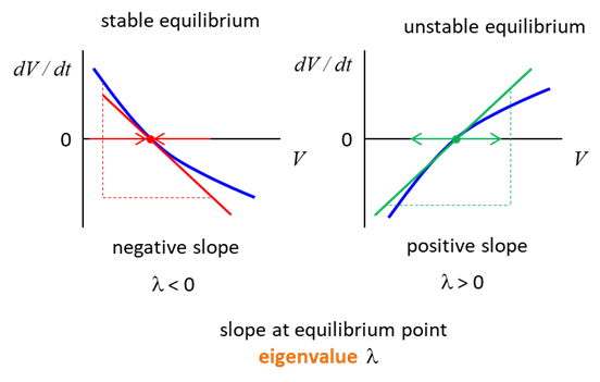
value of the membrane potential variable is exactly at equilibrium, then If the initial value
is near equilibrium, then the membrane potential may approach or diverge from
it. At an equilibrium point, when the slope of the curve At an equilibrium
point, when the slope of the curve
Fig. 12A. The slope of the curve The slope of the
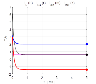
curve Figure 13 shows
the time evolution of the leak current IL, Na+ current INa the external current Iext,
and the combined current IL
+ INa.
The upper plot is for V0 = + 100 mV and the lower plot V0 = - 100
mV. At an equilibrium point the net current or combined current is equal to
the external current
Fig. 13. The time evolution of the
membrane currents: leak current IL, Na+ current INa the external current Iext,
and the combined current IL + INa . The upper plot is for V0 =
+ 100 mV (stable equilibrium + 38.8 mV) and the lower plot V0 = -
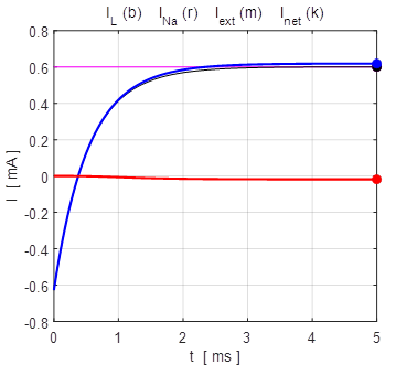
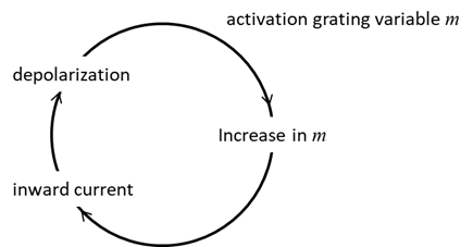
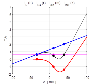
100 mV (stable equilibrium + 38.8 mV). np002.m Figure 14 shows the I-V characteristic plot: leak current IL, Na+ current INa, the external current Iext, and the combined current IL + INa. The shape I-V characteristic curve for the combined current IL + INa agrees very well with measured data from layer 5 pyramidal cells in a rat visual cortex. The slope of the I-V curve is equal to the conductance. For a region of membrane potentials where the slope has negative values then we have “negative conductance”. This negative conductance creates a positive feedback between the voltage VM and the gating variable minf (figure 10), and it plays an amplifying role in neurone dynamics. Such currents are referred to as amplifying currents.
Fig.
14. The I-V characteristic
plot: leak current IL, Na+
current INa the
external current Iext,
and the combined current IL + INa np002.m When the external current is set to zero, Iext = 0 A, there is only one stable equilibrium point, and the trajectory of the membrane potential is pulled a resting state.
Fig. 15.
All trajectories for different initial membrane potentials are
attracted to the single stable equilibrium point, VM = - 67 mV (monostability).
Fig. 16. There is only one point where The transition
between two stable states separated by a threshold is relevant to the
mechanism of excitability and generation of action potentials of many
neurones. In our Leak / fast Na+
model, the existence of the rest state is largely due to the leak current IL, while the
existence of the excited state is largely due to the persistent inward Na+
current INa. Small
(sub-threshold) perturbations leave the state variable in the attraction
domain of the rest state, while large (super-threshold) perturbations
initiate the regenerative process where the upstroke of an action potential, and the voltage variable becomes attracted to
the excited state.
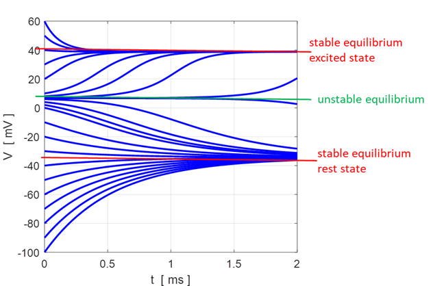
Fig.
17. Upstroke dynamics for the
generation of action potential for our Leak / fast Na+ model. The
model describes quite well the upstroke dynamics of layer 5 pyramidal
neurones. Iext = 0.60
mA
np002B.m Generation of the
action potential must be completed via repolarization that moves VM back to the rest
state. Typically, repolarization occurs because of a relatively slow
inactivation of Na+ current and/or slow activation of an outward K+
current, which are not taken into account our model. BIFURCATIONS A system is said to
undergo a bifurcation
when its qualitative behaviour changes. We can
investigate changing the external current injected into a neurone using our
leak / fast Na+ model. When the external
current is zero, all trajectories for initial membrane potentials are
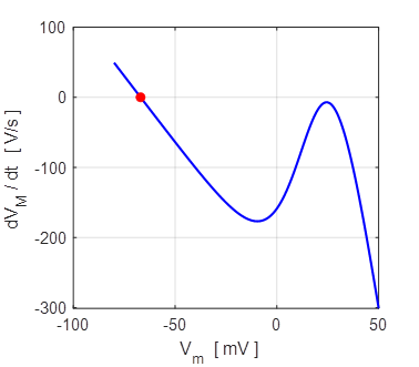
attracted to the rest state where VM = - 67 mV (figure 18).
Fig. 18. Iext = 0 mV There is only a single stable equilibrium point at the rest membrane potential VM
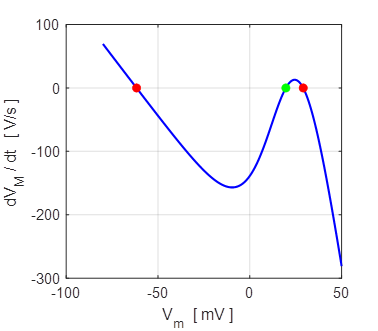
= - 67 mV. Monostable np002B.m When the external current is increased Iext = 0.1 mA, then the system is bistable with stable
equilibrium at -62 mV (rest state) and + 29 mV (excited state) as shown in
figure 19.
Fig. 19. Iext = 0.1 mA There are two stable equilibrium points: rest membrane potential
-62 mV and the excited state +29 mV. The unstable
equilibrium point is around +20 mV.
Bistable
np002B.m When the external current is greater than
about 0.9 mA, there is again only one stable equilibrium
point as shown in figure 20.
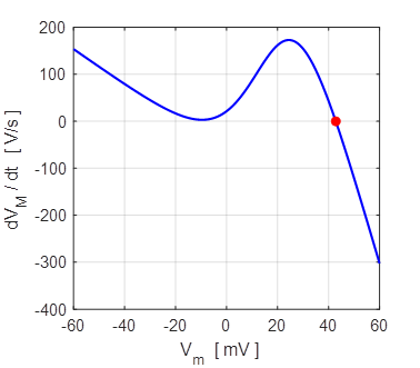
Fig. 20 Iext = 0.9 mV There is only a single stable equilibrium point at the excited state
membrane potential
VM
= 43 mV. Monostable
np002B.m We can clearly see that the qualitative
behaviour of our model depends upon the value of the external current. Iext = 0 mA, the system evolves to the resting
state. ~0.1 mA <
Iext < ~0.9 mA, the system
is bistable where the rest and excited states coexist. Iext > ~ 0.9 mA, the rest state no longer
exists because the leak current cannot cope with the large injected DC
injected current and the inward Na+ current. When Iext ~
0.9 mA a saddle-mode bifurcation exists since slight
variations in Iex results in the system evolving to
a bistable or monstable state. As Iext is increased, the EXAMPLES The examples given are based upon the
Exercises in Chapter 3 of the Izhikevich’s
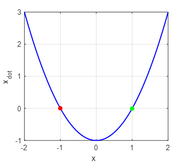
book. 1. Script np003.m System:
The red dot shows a stable equilibrium point and a green
dot an unstable
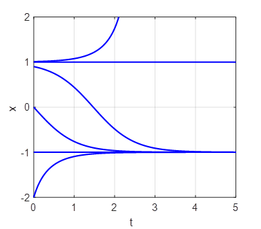
equilibrium point. For all initial values x < 1, the trajectory of the
system will evolve to the stable equilibrium point at x = -1. For all values of x > 1, the trajectory of the
system will diverge to infinity. The attraction domain corresponds to all
initial values x < 1. The eigenvalues are the roots of the function
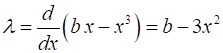
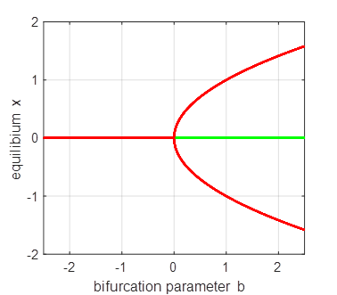
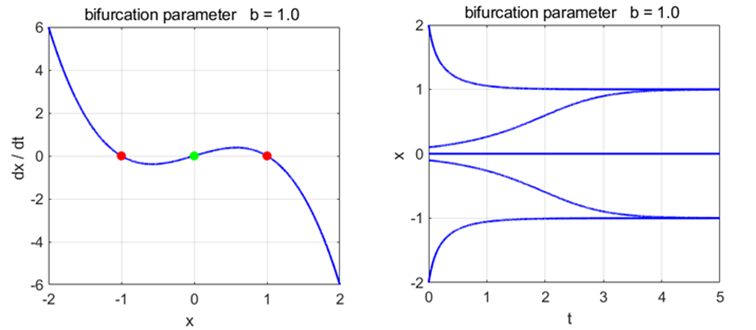
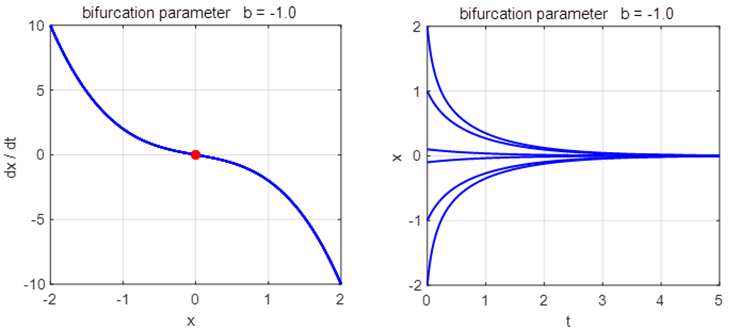
2. Script np003A.m System: The eigenvalues are
If If
Saddle-node
(fold) bifurcation diagram np003A.m The branch
Phase
Portrait and Time Evolution Plots: b = +1, 0, and -1 np003A.m |
|
|