Matlab Physics

FITZHUGH-NAGUMO MODEL FOR SPIKING NEURONS

Ian Cooper

Any comments, suggestions or corrections, please email me at

matlabvisualphysics@gmail.com

MATLAB

cnsFNA.m

The technique of phase plane analysis is used to model the action potentials generated by neurons with the Fitzhugh-Nagumo Model. The dynamics of the two- state variable system (membrane potential v and recovery variable w) can be explored. The function ode45 function is used to solve the pair of coupled differential equations. The variable y gives v and w. Most of the parameters are specified in the INPUT SECTION. For different models it may be necessary to make some changes to the Script. The results are displayed in as a phase space plot and a time evolution plot. By changing the parameters within the Script, you can investigate in detail the dynamics of the Fitzhugh-Nagumo model of a spiking neuron and explore all the essential aspects of the model.

The coupled pair of differential equation is solved using the ode45 function

% K use to pass variables to function FNode

K = [Iext; a; b; c];

% Solve differential equations using ode45

[t,y] = ode45(@(t,y) FNode(t,y,K), tSpanT,y0);

function dydt = FNode(t,y,K)

a = K(2); b = K(3); c = K(4); Iext = K(1);

%Iext = 0.003 * t;

%if t > 50; Iext = 0.5; end

%if t > 55; Iext = 0; end

dydt = [(y(1)-y(1)^3/3-y(2)+Iext); (1/c)*(y(1) + a - b*y(2))];

end

ACTION POTENTIALS

Nerve cells are separated from the extracellular region by a lipid bilayer membrane. When the cells aren’t conducting a signal, there is a potential difference of about -70 mV across the membrane (outside of the membrane the potential is taken as zero). This potential difference is known as the cell’s resting potential. On both sides of the nerve cell membrane, the concentrations of positive ions such as sodium, potassium and calcium and negatively chlorine ions and protein ions maintain the resting potential. When the cell receives an external stimulus, an action potential maybe evoked where the membrane potential spikes toward a positive value, in a process called depolarization, after which, repolarization occurs where the membrane potential resets back to the resting potential.

In one example, the concentration of the sodium ions at rest is much higher in the extracellular region than it is within the cell. The membrane contains gated channels that selectively allow the passage of ions though them. When the cell is stimulated, the sodium channels open and there is a rush of sodium ions into the cell. This sodium “current” raises the potential of the cell, resulting in depolarization. However, since the channel gates are voltage driven, the sodium gates close after a while. The potassium channels then open and an outbound potassium current flows, leading to the repolarization of the cell.

In 1952, Hodgkin and Huxley explained this mechanism of generating action potential through their mathematical model. While this was a great success in the mathematical modeling of biological phenomena, the Hodgkin-Huxley model is complicated. However, in 1961, R. Fitzhugh and J. Nagumo proposed a mathematical neuroscience model referred to as FitzHugh-Nagumo model. This model is a simpler version of the Hodgkin-Huxley model which demonstrates the spiking potentials in neurons and emulates the potential signals observed in a living organism’s excitable nerve cells. 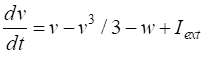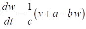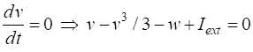The Fitzhugh-Nagumo model has only a few parameters and two coupled differential equations for the membrane potential, v, and the recovery variable w, which modulates v.

FITZHUGH-NAGUMO MODEL

The pair of coupled first order equations defining the Fitzhugh-Nagumo Model are

(1A)

(1B)

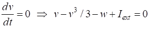
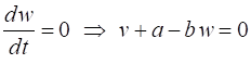
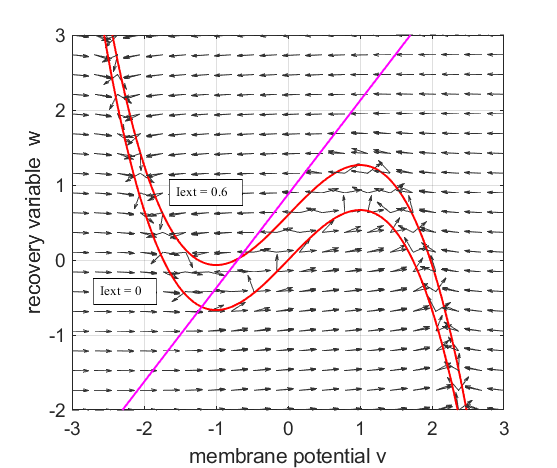
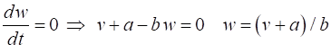
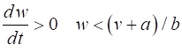
The variable v is a voltage-like membrane potential having cubic nonlinearity that allows regenerative self-excitation via a positive feedback and w is called the recovery variable having linear dynamics that provides a slower negative feedback. The parameter corresponds to a stimulus current. A positive current, corresponds to a current directed from outside the cell membrane to inside. The parameters a and b are controlling parameters of the system. The parameter c is responsible for the evolution of w being slower than the evolution of v.

The two nullclines in the v-w plane are given by

v-nullcline cubic polynomial

w-nullcline straight line

The intersection of the two nullclines gives the critical points (fixed equilibrium points) of the model. The slope of the straight-line is controlled by the two parameters a and b is such that the nullclines intersect at a single point, making it the system’s only fixed point. The critical point corresponds to the resting state of the neuron.

The parameter simply shifts v-nullcline up or down. Thus, changing modulates the position of the critical point so that different values of cause the critical point to be on the left, middle, or right part of the v-nullcline curve. The position of the critical point determines the dynamics of the membrane potential v. As the external stimulus current increases, the trajectory moves up, while the critical point moves to the right. If the stimulus current decrease, the trajectory moves down, and the critical point moves to the left. The trajectory is governed by the v-w vector field, shown by arrows pointing in the direction of increasing time (figures 1 and 2). The arrows indicating the vector field are normalized, so that they have unit length. The v-w trajectory is always tangential to the vector field described by the arrows. All quantities in the model are expressed in arbitrary units and not in S.I. units.

Fig. 1. The red curves are the v-nullcline and the magenta straight line is the w-nullcline. The intersection of the v-nullcline and the w-nullcline gives the single critical point of the system. An increase in the external current stimulus shifts the v-nullcine up and changes the position of the critical point. a = 0.7 b = 0.8 c = 12.5

cnsFNA.m The statement close all is commented out and a break point inserted before the trajectory is plotted. Then the Script is run for different values of .

We can estimate the coordinates of the critical point in v-w phase space by solving the equations numerically using the Matlab function vpasolve and then output the results in the Command Window.

(2A)

(2B)

% Critical point - output to Command Window

syms p

Sp = vpasolve(p-p^3/3-(p+0.7)/0.8 + Iext == 0,p,[-3 3]);

Sq = (Sp+a)/b;

disp('Critical point');

fprintf(' v_C = %2.2f\n', Sp);

disp(' ')

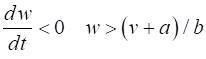
fprintf(' w_C = %2.2f\n', Sq);

DYNAMICS OF THE FITZHUGH-NAGUMO MODEL

To the left of the straight-line w-nullcline, the rate of change of w is negative and to the right it is positive;

left right

For the v-nullcline, above the line the rate of change of v is negative, while below the line is positive

above below

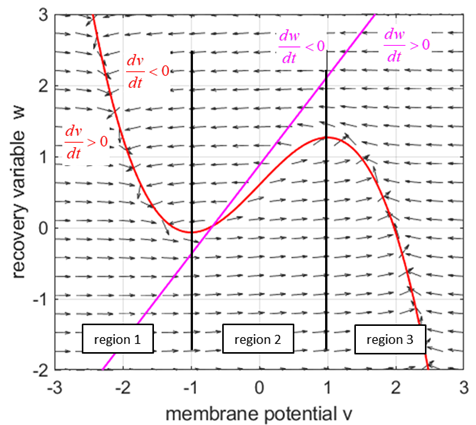
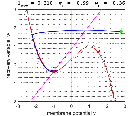
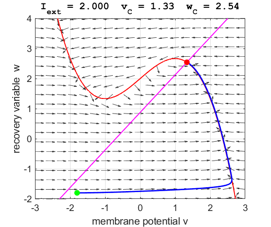
Fig. 2. Critical point is in region 2. The vector field (direction of the arrows) indicates the sign of and the sign of .

Small external stimulus currents

The critical point is in region 1. The state variables evolve to the critical point without exciting a spike in the potential v (figure 3).

Fig. 3A. The phase space trajectory is attracted to the critical point. The green dot gives the starts and the red dot gives the end of the trajectory.

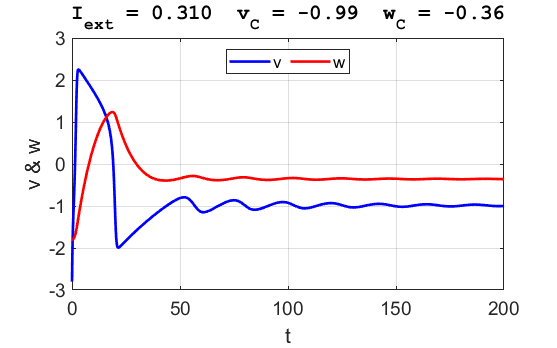
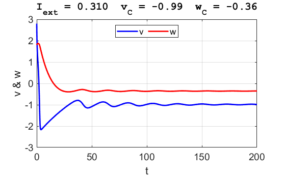
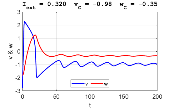
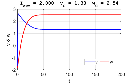
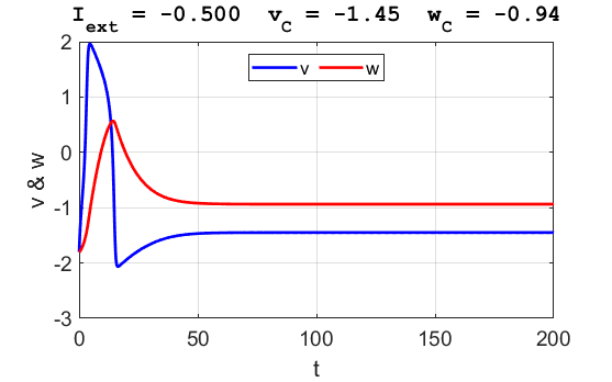
Fig. 3B. The time evolution of the two state variables. There are small oscillations which become quickly damped around critical point.

Fig. 3C. The phase space trajectory is attracted to the critical point. The green dot gives the starts and the red dot gives the end of the trajectory.

Fig. 3B. The time evolution of the two state variables. There are small oscillations which become quickly damped around critical point.

For an external current stimulus, , the critical point is at the boundary between regions 1 and 2. The trajectory oscillates around the critical point without an action potential being initiated (figure 4).

For weak current stimuli, there is a stable fixed equilibrium point.

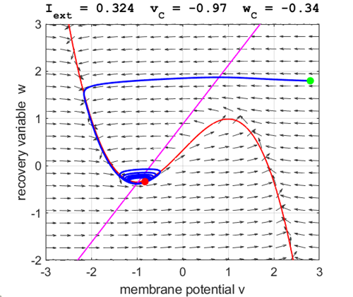
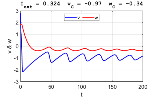
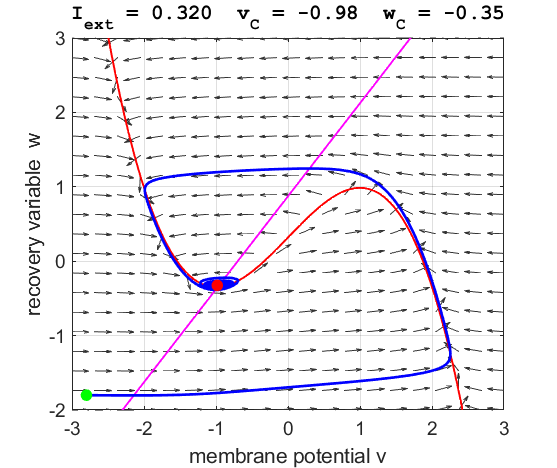
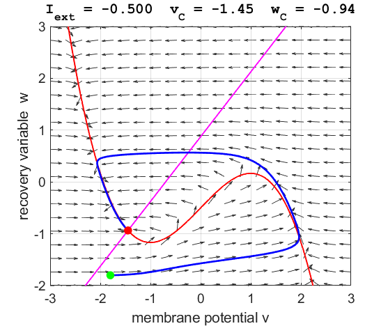
Fig. 4. The critical point is at the boundary of regions 1 and 2. The trajectory oscillates around the critical point without an action potential being produced.

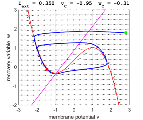
Intermediate external stimulus currents

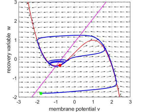
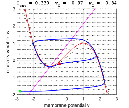
The critical point is in region 2 and is an unstable equilibrium point. A series of action potentials are generated. The neuron spikes repetitively, that is, the model exhibits periodic (tonic spiking) activity.

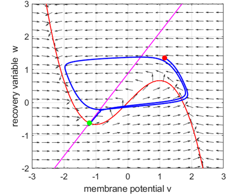
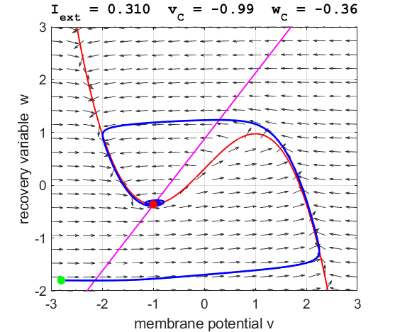
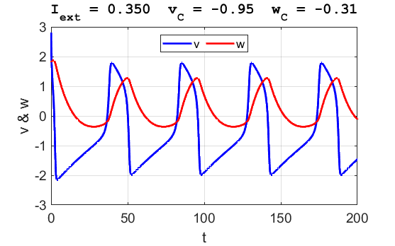
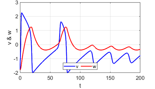
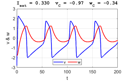
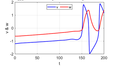
Fig. 5A. The critical point acts as a center and is in region 2. The trajectory forms closed loops around the critical point which results in the repetitive spiking of the neuron. At the start, v decreases and w remains nearly unchanged. When the trajectory approaches the v-nullcline, and the trajectory follows the v-nullcline as w rapidly decreases until the w-nullcline is reached where and the evolution of v dominates and the curve becomes horizontal once again. This continues until the trajectory hits the right part of the v-nullcline. The trajectory begins to hug the v-nullcline and starts a slow upward journey. Thus, the trajectory sweeps out a closed orbit and never hits the critical point and therefore keeps repeating itself.

Fig. 5B. A series of action potentials are produced. The fixed equilibrium point is unstable and leads to tonic firing of the neuron.

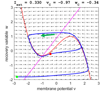
Fig. 5C. The critical point acts as a center. The trajectory forms closed loops around the critical point which results in the repetitive spiking of the neuron.

It is possible to get a single spike generated by carefully adjusting the value . Figure 5D shows the simulation for

Fig. 5D. A single spike is produced when .

We can demonstrate the concept of the Hopf bifurcation. A Hopf bifurcation occurs when there is a qualitative change in the system dynamics as the system parameters are varied. When , the phase space trajectory is attracted to the resting point, i.e., the stable fixed equilibrium point (critical point) as shown in figure 5E. However, when there is a slight increase in the current stimulation, , the critical point becomes unstable. The phase space trajectory is attracted to the limit cycle and a periodic spiking of the neuron occurs (figure 5F).

Fig. 5E. The phase space trajectory is attracted to the critical point.

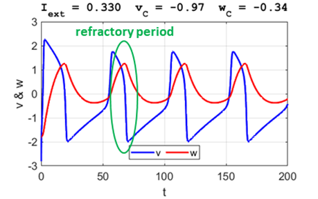
Fig. 5F. The phase space trajectory is attracted to the limit cycle and the neuron spikes periodically.

After a spike, the neuron returns to its resting state during the refractory period where the system is indifferent to any external stimuli (figure 5G).

refractory period

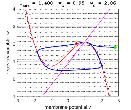
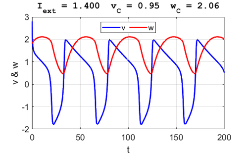
Fig. 5G. The phase space trajectory is attracted to the limit cycle and the neuron spikes periodically. After a spike, the neuron returns to its resting state during the refractory period where the system is indifferent to any external stimuli.

Large external stimulus currents

Fig. 6. The critical point is in region 3. The trajectory is attracted to the critical point. No action potentials are generated. At the start , v evolves faster than w, that is, v increases rapidly while w remains virtually unchanged (near-horizontal part of the v-w trajectory). As the trajectory approaches the v-nullcline, the rate of change of v slows down and w becomes more prominent. Since is still positive, w must increase, and the trajectory moves upwards. The fixed point then attracts this curve and the evolution ends at the fixed point.

SUMMARY

The Fitzhugh-Nagumo model explains the absence of all-or-none spikes in the Hodgkin-Huxley model in response to weak stimuli that result in small-amplitude trajectories that correspond to subthreshold responses. Stronger stimuli result in intermediate-amplitude trajectories that correspond to partial-amplitude spikes whereas strong stimuli result in large-amplitude trajectories that correspond to suprathreshold response producing the firing of spikes.

The, Fitzhugh-Nagumo model does not have a well-defined firing threshold, like the Hodgkin-Huxley model. This feature is the consequence of the absence of all-or-none responses, and it is related, from the mathematical point of view, to the absence of a saddle equilibrium.

The FitzHugh-Nagumo model explains the excitation block phenomenon, i.e., the cessation of repetitive spiking as the amplitude of the stimulus current increases. When is small or zero, the equilibrium (intersection of nullclines) is in region 1 and on the left (stable) branch of v-nullcline, and the model is resting. Increasing shifts the nullcline upward and the equilibrium slides onto region 2, the middle (unstable) branch of the nullcline. The model exhibits periodic spiking activity in this case. Increasing the stimulus further shifts the equilibrium to region 3, the right (stable) branch of the N-shaped nullcline, and the oscillations are blocked by the excitation. The precise mathematical mechanism involves appearance and disappearance of a limit cycle attractor.

The Fitzhugh-Nagumo model explains the phenomenon of post-inhibitory (rebound) spikes, called anodal break excitation. As the stimulus becomes negative (hyperpolarization), the resting state shifts to the left. As the system is released from hyperpolarization (anodal break), the trajectory starts from a point far below the resting state and makes a large-amplitude excursion, i.e., fires a transient spike, and then returns to the resting state as shown in figure 7.

Fig. 7. Anodal break excitation (post-inhibitory rebound spike) in the Fitzhugh-Nagumo model.

The FitzHugh-Nagumo model explained the dynamical mechanism of spike accommodation in Hodgkin-Huxley model. When stimulation strength increases slowly, the neuron remains quiescent. The resting equilibrium of the Fitzhugh-Nagumo model shifts slowly to the right, and the state of the system follows it smoothly without firing spikes until the current stimulus results in repetitive spiking of the neuron (figure 8).

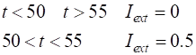
Fig. 8. Spike accommodation to slowly increasing stimulus in the Fitzhugh-Nagumo model. The external current stimulus used was .

In contrast, when the stimulation is increased abruptly, even by a smaller amount, the trajectory cannot go directly to the new resting state but fires a transient spike (figure 9).

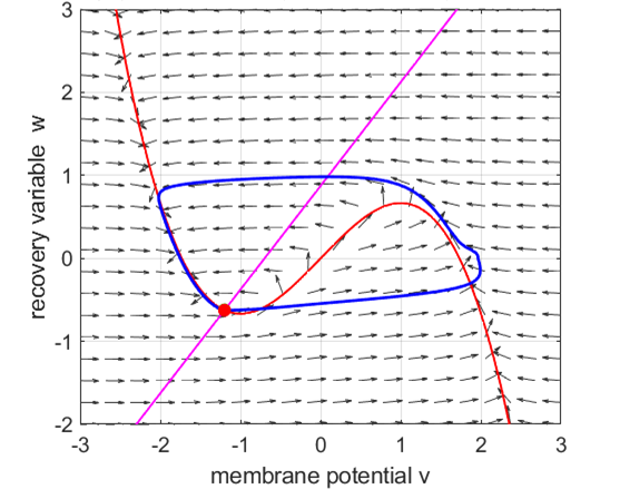
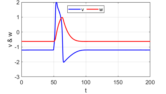
Fig. 9. Spike accommodation: response to a short current stimulus. The current pulse results in the firing of a transient spike, like the post-inhibitory (rebound) response. The neuron is initially in a resting state.

Figures 8 and 9 were produced by making changes to the function used in the ode45 call.

Changes to were made by commenting / uncommenting lines within the function.

function dydt = FNode(t,y,K)

a = K(2); b = K(3); c = K(4); Iext = K(1);

%Iext = 0.003 * t;

if t > 50; Iext = 0.5; end

if t > 55; Iext = 0; end

dydt = [(y(1)-y(1)^3/3-y(2)+Iext);(1/c)*(y(1)+a-b*y(2))];

end