|
|
AN INTRODUCTION TO
PERCOLATION THEORY A MATLAB
SIMULATION Matlab mscript percolation.m |
|
|
|
||
|
This paper describes a simple
Matlab simulation on site percolation
in which you can generate and visualize percolation clusters using the
mscript percoloation.m. We will consider a square lattice
of linear dimension L. The number of lattice sites is L x L. Each lattice
site maybe occupied (1) or
unoccupied or empty (0).
Each site is occupied independently of its neighbors with probability p.
The occupied sites form clusters in which sites maybe or may not
connected to their nearest neighbors. Each occupied state belongs to a unique
cluster. To investigate percolation theory,
we generate a L × L matrix of random numbers and then a lattice site is
occupied if the random number is less than the assigned probability p. If the probability p is small then
only small clusters are likely to be formed and if p is large, then most of
the lattice sites will be occupied. When p ~ 1 you would expect the formation
of a large cluster that extends from one edge of the lattice to the other.
Such a cluster is called a spanning cluster. There exists a threshold
probability pc such
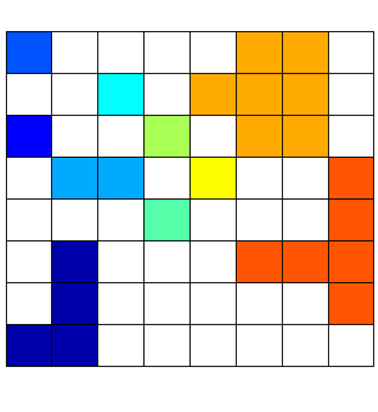
that An important characteristic of
percolation is connectedness and we can relate this concept to phase
transitions. We see
that a well-defied value of the parameter pc determines whether a
spanning cluster exists or does not exist: as pc is increased
there will be a transition from zero spanning clusters to a spanning cluster
and this represents a type of phase transition. For example, consider the
electrical conductivity of a material made from a composite material of
metallic and insulating materials. The sample is non-conducting when the
percentage of the metallic material is small, however, in increasing the
percentage of the metallic material, a sharp transition occurs from the
non-conducting state to the conducting state when there is a connected
pathway of metallic material (a spanning cluster). There are many
applications of percolation theory in modelling physical systems such as
magnetic materials, behavior of gels and spread of disease in a population. It is necessary to label each
cluster so that we can investigate the percolation. The [2D] matrix u of
dimensions L x L is the percolation matrix and each element of the matrix is
either 1 (occupied site) or 0 (empty site). The Matlab function bwlabel
can be used to assigned the labels to each cluster [cls,numC] = bwlabel(u,4); Where cls
are the labels attached to each element of u and numC is the number of clusters. You can familiarize yourself with
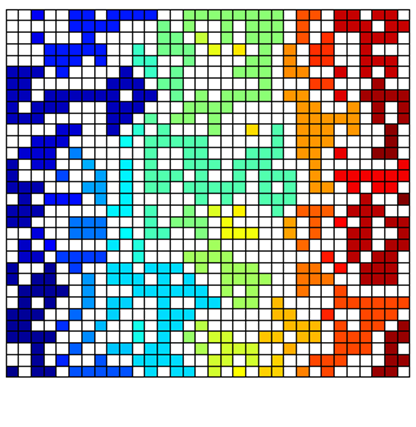
the labeling by viewing the Matlab help system on bwlabel in the image analysis toolbox. We also can examine the percolation
matrix and clusters directly by mapping the labels onto a color-map using the
function label2rgb. |
||
|
clsT = zeros(L,L); for c = 1 : L
clsT(c,:) = cls(L+1-c,:); end figure(2) set(gcf,'units','normalized','position',[0.35 0.52 0.23 0.32]); img = label2rgb(clsT); image(img); axis off |
||
|
The mscript percolation.m can be used to calculate the
following quantities ·
Number of occupied
sites: nOSites ·
Simulation probability
of a site being occupied: pOSites (can compare with
probability p) ·
Cluster labels: cls and number of clusters: numC ·
Cluster size - number
of occupied sites in each cluster: nC ·
Counter – 1 to
maximum number of occupied sites in clusters: s ·
Number of clusters with
s occupied sites: nS ·
Probability that an
occupied site chosen at random is part of an s-site cluster: probROS ·
Mean cluster size
(average number of occupied sites for the clusters): S or meanclustersize ·
Spanning clusters: isSpanX and isSpanY (in finding spanning
clusters you only need to check the cluster numbers at the edges of the
lattice. You should run the mscript many times to
calculate the average values of many of the above quantities and by carefully
incrementing the value of the probability p you can find the threshold
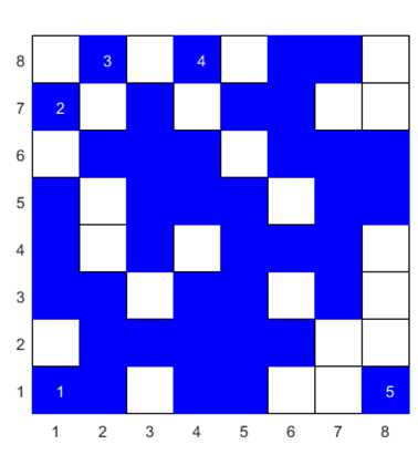
probability pc. Figures 1 and 2 show the results of two
simulations extracted from the Matlab Figure Windows and the Command Window
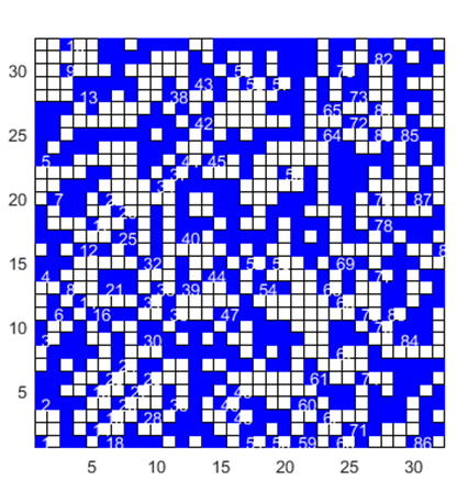
for L = 8 and different p values: p = 0.30 and p = 0.60. Figure 3 shows the plots for
L = 32
and p = 0.50. |
||
|
|
|
|
|
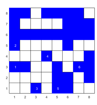
Fig. 1. Zero spanning
clusters. Linear dimension L = 8 Total number of sites nSties
= 64 Probability of a site being occupied p = 0.30 Number of occupied sites nOSites = 25 Simulation: probability of a site being occupied pOSites = 0.39 Number of clusters numC = 10
Cluster Size: number of occupied sites in each cluster nC 4 1 1 2 1 1 1 1 7 6 Cluster Size Distribution s nS probROS 1 6 0.600 2 1 0.100 3 0 0.000 4 1 0.100 5 0 0.000 6 1 0.100 7 1 0.100 Mean Cluster Size S: sites / clusters / prob S = mean(nC) = 2.500 S = SUM(s .* probROS) = 2.500 Spanning clusters = 1 cluster # rows cols
1
0 0
2
0 0
3
0 0
4
0 0
5
0 0 6 0 0
7
0 0
8
0 0
9
0 0 10 0
0 |
||
|
|
|
|
|
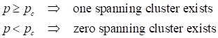
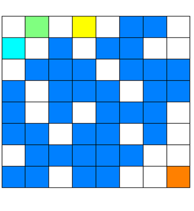
Fig. 2. One spanning
cluster. Linear
dimension L = 8 Total number
of sites nSties
= 64 Probability
of a site being occupied p
= 0.60 Number of
occupied sites nOSites = 40 Simulation:
probability of a site being occupied pOSites = 0.63
Number of
clusters numC
= 5 Cluster
Size: number of occupied sites in each cluster nC 36 1 1 1 1 Cluster Size
Distribution s nS
probROS 1 4 0.800 2 0 0.000 3 0 0.000 4 0 0.000 5 0 0.000 6 0 0.000 7 0 0.000 8 0 0.000 9 0 0.000 10 0 0.000 11 0 0.000 12 0 0.000 13 0 0.000 14 0 0.000 15 0 0.000 16 0 0.000 17 0 0.000 18 0 0.000 19 0 0.000 20 0 0.000 21 0 0.000 22 0 0.000 23 0 0.000 24 0 0.000 25 0 0.000 26 0 0.000 27 0 0.000 28 0 0.000 29 0 0.000 30 0 0.000 31 0 0.000 32 0 0.000 33 0 0.000 34 0 0.000 35 0 0.000 36 1 0.200 Mean Cluster
Size S: sites / clusters / prob S = mean(nC) = 8.000 S = SUM(s .*
probROS) = 8.000 Spanning
clusters = 1 cluster
# rows cols 1 1 1 2 0 0 3 0 0 4 0 0 5 0 0 |
||
|
|
|
|
|
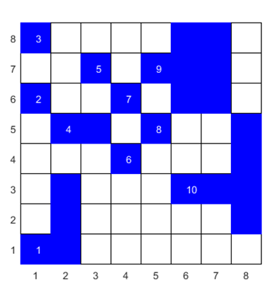
Fig. 3. L = 32 and p = 0.50. |
||
|
REFERENCES Harvey Gould and Jan Tobochnik, An Introduction to Computer Simulation
Methods: Applications to Physical Systems Part2, Addison-Wesley 1988. There are many excellent resources on the web for Percolation Theory,
simply search percolation
theory |
||
|
|
||